The Digested Read: Every PhD in Health Informatics

By rmhipmt, on 10 November 2010

No one has time to read other people’s PhD theses. So, inspired by the Guardian’s Digested Read column, we’ve decided to publish succinct – very succinct – summaries of the major categories of Health Informatics PhD.

Today, in issue 1 of the series, we deal with classification problems.

Using a Fashionable New Computer Science Paradigm to Classify Cases of an Important Disease

Background
This disease is a major health problem and one where diagnostic or management errors can occur. Previous attempts to apply computers to classify cases of this disease have achieved promising results (classification accuracy of over 70% is commonly claimed) but haven’t yet led to clinical take-up. A fashionable new computer science paradigm seems to offer an exciting and novel approach to this problem.

Method
An innovative algorithm based on the fashionable new computer science paradigm was implemented by the candidate. Applying the algorithm to a publicly available dataset with questionable ground truth achieved a classification accuracy of barely more than 60%. Successive, increasingly desperate, and, in the end, almost random modifications allow a classification accuracy of nearly 70% to be claimed.

Results
A new, but disappointingly small, dataset was collected in collaboration with the local clinical team. On this dataset, the modified algorithm achieved an accuracy of just less than 60% when tested against the consensus opinion of clinicians. Closer analysis identified a subset of interesting cases where junior clinicians only achieved agreement levels of 58% when assessed against each other.

Conclusions
The application of the fashionable new computer science paradigm to this important disease seems highly promising.

Java example code of common similarity algorithms, used in data mining

By rmhiajd, on 28 June 2010

I am currently researching record linkage techniques and so had to remind myself of the some of the algorithms used in and around the area to help evaluate the products I have at my disposal. This work has been undertaken as part of the DHICE project at UCL, funded by the Wellcome Trust.

My typical approach to understanding algorithms is to code them up and so I am then able to “play” with them. In the process of researching each technique I noticed in most cases there was only pseudo code available. So I have decided to share the Java examples of the following algorithms:

Levenshtein
Damerau Levenshtein
Hamming
Jaro Winkler
Smith Waterman
N-Gram
Markov Chain

For each algorithm, I will provide a very basic description and then the Java code which you are free to play with, further to this I will provide links to the wikipedia entry for the algorithm and any other site I have sourced. Each piece of code is based around the explanation in Wikipedia and has been tested against the examples provided by each Wikipedia article and/or other sites referenced. There is no warranty provided with this code, any changes / enhancements / corrections / or use of this code should be attributed to CHIME, UCL and shared with the community.

Levenshtein

The purpose of this algorithm is to measure the difference between two sequences/strings. It is based around the number of changes required to make one string equal to the other.

It is aimed at short strings, it usage is spell checkers, optical character recognition, etc.

Wikipedia entry can be found here:

[java]

public class Levenshtein
{
private String compOne;
private String compTwo;
private int[][] matrix;
private Boolean calculated = false;

public Levenshtein(String one, String two)
{
compOne = one;
compTwo = two;
}

public int getSimilarity()
{
if (!calculated)
{
setupMatrix();
}
return matrix[compOne.length()][compTwo.length()];
}

public int[][] getMatrix()
{
setupMatrix();
return matrix;
}

private void setupMatrix()
{
matrix = new int[compOne.length()+1][compTwo.length()+1];

for (int i = 0; i <= compOne.length(); i++)
{
matrix[i][0] = i;
}

for (int j = 0; j <= compTwo.length(); j++)
{
matrix[0][j] = j;
}

for (int i = 1; i < matrix.length; i++)
{
for (int j = 1; j < matrix[i].length; j++)
{
if (compOne.charAt(i-1) == compTwo.charAt(j-1))
{
matrix[i][j] = matrix[i-1][j-1];
}
else
{
int minimum = Integer.MAX_VALUE;
if ((matrix[i-1][j])+1 < minimum)
{
minimum = (matrix[i-1][j])+1;
}

if ((matrix[i][j-1])+1 < minimum)
{
minimum = (matrix[i][j-1])+1;
}

if ((matrix[i-1][j-1])+1 < minimum)
{
minimum = (matrix[i-1][j-1])+1;
}

matrix[i][j] = minimum;
}
}
}
calculated = true;
displayMatrix();
}

private void displayMatrix()
{
System.out.println(” “+compOne);
for (int y = 0; y <= compTwo.length(); y++)
{
if (y-1 < 0) System.out.print(” “); else System.out.print(compTwo.charAt(y-1));
for (int x = 0; x <= compOne.length(); x++)
{
System.out.print(matrix[x][y]);
}
System.out.println();
}
}
}
[/java]

Damerau Levenshtein

Similar to Levenshtein, Damerau-Levenshtein also calculates the distances between two strings. It based around comparing two string and counting the number of insertions, deletions, and substitution of single characters, and transposition of two characters.

This was, originally, aimed at spell checkers, it is also used for DNA sequences.

Wikipedia entry found be here:

[java]

public class DamerauLevenshtein
{
private String compOne;
private String compTwo;
private int[][] matrix;
private Boolean calculated = false;

public DamerauLevenshtein(String a, String b)
{
if ((a.length() > 0 || !a.isEmpty()) || (b.length() > 0 || !b.isEmpty()))
{
compOne = a;
compTwo = b;
}
}

public int[][] getMatrix()
{
setupMatrix();
return matrix;
}

public int getSimilarity()
{
if (!calculated) setupMatrix();

return matrix[compOne.length()][compTwo.length()];
}

private void setupMatrix()
{
int cost = -1;
int del, sub, ins;

matrix = new int[compOne.length()+1][compTwo.length()+1];

for (int i = 0; i <= compOne.length(); i++)
{
matrix[i][0] = i;
}

for (int i = 0; i <= compTwo.length(); i++)
{
matrix[0][i] = i;
}

for (int i = 1; i <= compOne.length(); i++)
{
for (int j = 1; j <= compTwo.length(); j++)
{
if (compOne.charAt(i-1) == compTwo.charAt(j-1))
{
cost = 0;
}
else
{
cost = 1;
}

del = matrix[i-1][j]+1;
ins = matrix[i][j-1]+1;
sub = matrix[i-1][j-1]+cost;

matrix[i][j] = minimum(del,ins,sub);

if ((i > 1) && (j > 1) && (compOne.charAt(i-1) == compTwo.charAt(j-2)) && (compOne.charAt(i-2) == compTwo.charAt(j-1)))
{
matrix[i][j] = minimum(matrix[i][j], matrix[i-2][j-2]+cost);
}
}
}

calculated = true;
displayMatrix();
}

private void displayMatrix()
{
System.out.println(” “+compOne);
for (int y = 0; y <= compTwo.length(); y++)
{
if (y-1 < 0) System.out.print(” “); else System.out.print(compTwo.charAt(y-1));
for (int x = 0; x <= compOne.length(); x++)
{
System.out.print(matrix[x][y]);
}
System.out.println();
}
}

private int minimum(int d, int i, int s)
{
int m = Integer.MAX_VALUE;

if (d < m) m = d;
if (i < m) m = i;
if (s < m) m = s;

return m;
}

private int minimum(int d, int t)
{
int m = Integer.MAX_VALUE;

if (d < m) m = d;
if (t < m) m = t;

return m;
}
}
[/java]

Hamming

This algorithm calculates the distance between two strings, however they have to be of equal length.

It measures the minimum number of substitutions for the two strings to be equal.

It is used in telecommunication (also know as signal distance), it is also used in systematics as a measure of genetic distance.

Wikipedia entry can be found here:

[java]

public class Hamming
{
private String compOne;
private String compTwo;

public Hamming(String one, String two)
{
compOne = one;
compTwo = two;
}

public int getHammingDistance()
{
if (compOne.length() != compTwo.length())
{
return -1;
}

int counter = 0;

for (int i = 0; i < compOne.length(); i++)
{
if (compOne.charAt(i) != compTwo.charAt(i)) counter++;
}

return counter;
}

///
// Hamming distance works best with binary comparisons, this function takes a string arrary of binary
// values and returns the minimum distance value
///
public int minDistance(String[] numbers)
{
int minDistance = Integer.MAX_VALUE;

if (checkConstraints(numbers))
{
for (int i = 1; i < numbers.length; i++)
{
int counter = 0;
for (int j = 1; j <= numbers[i].length(); j++)
{
if (numbers[i-1].charAt(j-1) != numbers[i].charAt(j-1))
{
counter++;
}
}

if (counter == 0) return counter;
if (counter < minDistance) minDistance = counter;
}
}
else
{
return -1;
}

return minDistance;
}

private Boolean checkConstraints(String[] numbers)
{
if (numbers.length > 1 && numbers.length <=50)
{
int prevLength = -1;
for (int i = 0; i < numbers.length; i++)
{
if (numbers[i].length() > 0 && numbers[i].length() <= 50)
{
if (prevLength == -1)
{
prevLength = numbers[i].length();
}
else
{
if (prevLength != numbers[i].length())
{
return false;
}
}

for (int j = 0; j < numbers[i].length(); j++)
{
if (numbers[i].charAt(j) != ‘0’ && numbers[i].charAt(j) != ‘1’)
{
return false;
}
}
}
else
{
return false;
}
}
}
else
{
return false;
}

return true;
}
}
[/java]

Jaro Winkler

This algorithm is purposely designed for record linkage, it was designed for linking short strings. It calculates a normalised score on the similarity between two strings.

The calculation is based on the number of matching characters held within the string and the number of transpositions.

The wikipedia entry can be found here, the other source was lingpipe:

[java]

public class JaroWinkler
{
private String compOne;
private String compTwo;

private String theMatchA = “”;
private String theMatchB = “”;
private int mRange = -1;

public JaroWinkler()
{
}

public JaroWinkler(String s1, String s2)
{
compOne = s1;
compTwo = s2;
}

public double getSimilarity(String s1, String s2)
{
compOne = s1;
compTwo = s2;

mRange = Math.max(compOne.length(), compTwo.length()) / 2 – 1;

double res = -1;

int m = getMatch();
int t = 0;
if (getMissMatch(compTwo,compOne) > 0)
{
t = (getMissMatch(compOne,compTwo) / getMissMatch(compTwo,compOne));
}

int l1 = compOne.length();
int l2 = compTwo.length();

double f = 0.3333;
double mt = (double)(m-t)/m;
double jw = f * ((double)m/l1+(double)m/l2+(double)mt);
res = jw + getCommonPrefix(compOne,compTwo) * (0.1*(1.0 – jw));

return res;
}

private int getMatch()
{

theMatchA = “”;
theMatchB = “”;

int matches = 0;

for (int i = 0; i < compOne.length(); i++)
{
//Look backward
int counter = 0;
while(counter <= mRange && i >= 0 && counter <= i)
{
if (compOne.charAt(i) == compTwo.charAt(i – counter))
{
matches++;
theMatchA = theMatchA + compOne.charAt(i);
theMatchB = theMatchB + compTwo.charAt(i);
}
counter++;
}

//Look forward
counter = 1;
while(counter <= mRange && i < compTwo.length() && counter + i < compTwo.length())
{
if (compOne.charAt(i) == compTwo.charAt(i + counter))
{
matches++;
theMatchA = theMatchA + compOne.charAt(i);
theMatchB = theMatchB + compTwo.charAt(i);
}
counter++;
}
}
return matches;
}

private int getMissMatch(String s1, String s2)
{
int transPositions = 0;

for (int i = 0; i < theMatchA.length(); i++)
{
//Look Backward
int counter = 0;
while(counter <= mRange && i >= 0 && counter <= i)
{
if (theMatchA.charAt(i) == theMatchB.charAt(i – counter) && counter > 0)
{
transPositions++;
}
counter++;
}

//Look forward
counter = 1;
while(counter <= mRange && i < theMatchB.length() && (counter + i) < theMatchB.length())
{
if (theMatchA.charAt(i) == theMatchB.charAt(i + counter) && counter > 0)
{
transPositions++;
}
counter++;
}
}
return transPositions;
}

private int getCommonPrefix(String compOne, String compTwo)
{
int cp = 0;
for (int i = 0; i < 4; i++)
{
if (compOne.charAt(i) == compTwo.charAt(i)) cp++;
}
return cp;
}
}
[/java]

N-Gram

An algorithm to calculate the probability of the next term based on the previous n terms. It is used in speech recognition, phonemes, language recognition etc.

Wikipedia entry can be found here. Wikipedia, in this case, is a little limited on either pseudo code or an algorithm. In this case I referenced the following presentation (Slides 27/28) from CRULP talking about different algorithms used in spell checking. Also, further reading can be found in Chapter 6 of Christopher D Manning and Hinrich Schutze’s book Foundations of Statistical Natural Language Processing. N-Gram are very similar to Markov models.

Here is the code:

[java]

public class Ngram
{
private class result
{
private String theWord;
private int theCount;

public result(String w, int c)
{
theWord = w;
theCount = c;
}

public void setTheCount(int c)
{
theCount = c;
}

public String getTheWord()
{
return theWord;
}

public int getTheCount()
{
return theCount;
}
}

private List<result> results;

public Ngram()
{
results = new ArrayList<result>();
}
public Ngram(String str, int n)
{

}

public double getSimilarity(String wordOne, String wordTwo, int n)
{
List<result> res1 = processString(wordOne, n);
//displayResult(res1);
List<result> res2 = processString(wordTwo, n);
//displayResult(res2);
int c = common(res1,res2);
int u = union(res1,res2);
double sim = (double)c/(double)u;

return sim;
}

private int common(List<result> One, List<result> Two)
{
int res = 0;

for (int i = 0; i < One.size(); i++)
{
for (int j = 0; j < Two.size(); j++)
{
if (One.get(i).theWord.equalsIgnoreCase(Two.get(j).theWord)) res++;
}
}

return res;
}

private int union(List<result> One, List<result> Two)
{
List<result> t = One;

for (int i = 0; i < Two.size(); i++)
{
int pos = -1;
boolean found = false;
for (int j = 0; j < t.size() && !found; j++)
{
if (Two.get(i).theWord.equalsIgnoreCase(t.get(j).theWord))
{
found = true;
}
pos = j;
}

if (!found)
{
result r = Two.get(i);
t.add(r);
}
}

return t.size();
}

private List<result> processString(String c, int n)
{
List<result> t = new ArrayList<result>();

String spacer = “”;
for (int i = 0; i < n-1; i++)
{
spacer = spacer + “%”;
}
c = spacer + c + spacer;

for (int i = 0; i < c.length(); i++)
{
if (i <= (c.length() – n))
{
if (contains(c.substring(i, n+i)) > 0)
{
t.get(i).setTheCount(results.get(i).getTheCount()+1);
}
else
{
t.add(new result(c.substring(i,n+i),1));
}
}
}
return t;
}

private int contains(String c)
{
for (int i = 0; i < results.size(); i++)
{
if (results.get(i).theWord.equalsIgnoreCase(c))
return i;
}
return 0;
}

private void displayResult(List<result> d)
{
for (int i = 0; i < d.size(); i++)
{
System.out.println(d.get(i).theWord+” occurred “+d.get(i).theCount+” times”);
}
}
}
[/java]

Markov Chain

The Markov Chain model calculates the probability of the next letter occurring in a sequence based on the previous n characters.

They are used in a multitude of areas, including data compression, entropy encoding, and pattern recognition.

The wikipedia entry can be found here. I based my algorithm off of an excellent explanation found here, provided by Rutgers as part of their course Discrete and Probabilistic Models in Biology.

Warning, I think this document has a couple of mistakes in the matrix on page 10 (the counting of A,C,G,T), or I am mistaken?

For this code, the final part which is needed is a method which gives the probability of a sequence, that is you pass in a sequence and it returns the probability of this sequence based on the matrix it has calculated.

The code:

[java]
public class Markov
{

private class similarities
{
private char c;
private int count;

public similarities(char a, int b)
{
c = a;
count = b;
}

public char getC()
{
return c;
}

public int getCount()
{
return count;
}

public void setCount(int a)
{
count = a;
}

public void increaseCount()
{
count++;
}
}

private List<similarities> entries;
private List<String> axies;
private double[][] matrix;

public Markov()
{
entries = new ArrayList();
axies = new ArrayList();
}

public void getSimilarity(List<String> s)
{
String temp = new String();
for (int i = 0; i < s.size(); i++)
{
if (temp.length() > 0)
{
temp = temp + ” ” + s.get(i);
}
else temp = s.get(i);

}
setupAxis(temp);
compareCharsAgainstAxis(temp);

display();

for (int i = 0; i < matrix.length; i++)
{
double line = getLineValue(i);
for (int j = 0; j < matrix[i].length; j++)
{
double t = matrix[i][j];

matrix[i][j] = t / line;
}
}

display();
}

private void compareCharsAgainstAxis(String s)
{
matrix = new double[axies.size()][axies.size()];
String comparison = “”;
String test = s;

for (int h = 0; h < test.length(); h++)
{
int end = test.indexOf(” “);
if (end > 0)
{
comparison = test.substring(0,end);
}
else
{
comparison = test.substring(0,test.length());
end = test.length()-1;
}
test = test.substring(end+1,test.length());

for (int i = 1; i < comparison.length(); i++)
{
for (int j = 0; j < axies.size(); j++)
{
for (int k = 0; k < axies.size(); k++)
{
if (String.valueOf(comparison.charAt(i-1)).equalsIgnoreCase(axies.get(j)) && String.valueOf(comparison.charAt(i)).equalsIgnoreCase(axies.get(k)))
{
matrix[j][k]++;
}
}
}
}
}

}
private void setupAxis(String temp)
{
for (int j = 0; j < temp.length(); j++)
{
boolean found = false;

for (int k = 0; k < axies.size() && !found; k++)
{
if (String.valueOf(temp.charAt(j)).equalsIgnoreCase(axies.get(k)))
{
found = true;
}
}

if (!found)
{
if (temp.charAt(j) > 32)
{
axies.add(String.valueOf(temp.charAt(j)));
}
}
}
}

private double getTotalValue()
{
double sum = 0;
for (int i = 0; i < matrix.length; i++)
{
for (int j = 0; j < matrix[i].length; j++)
{
double t = matrix[i][j];
sum = sum + t;
}
}
return sum;
}

private double getLineValue(int line)
{
double sum = 0;
for (int i = 0; i < matrix[line].length; i++)
{
double t = matrix[line][i];
sum = sum + t;
}
return sum;
}

private void display()
{
System.out.println(“Sum of matrix is “+getTotalValue());
System.out.println(“Sum of line 1 = “+getLineValue(3));

System.out.print(” “);
for (int j = 0; j < axies.size(); j++)
{
System.out.print(axies.get(j)+” “);
}
System.out.println();
for (int i = 0; i < matrix.length; i++)
{
System.out.print(axies.get(i)+” “);
for (int j = 0; j < matrix[i].length; j++)
{
System.out.print(matrix[i][j]+” “);
}
System.out.println();
}
}
}
[/java]

I hope this proves useful?

What’s the evidence?

By rmhipmt, on 25 June 2010

Two things happened yesterday that made me think about how we assess the evidence for and against a hypothesis. The first was a radio debate in which a politician – known to his detractors as the Right Hon. member for Holland & Barrett – was arguing with a scientist about what we could infer from three selected studies of homeopathy. The second was a session with MSc students talking about how to evaluate and present the conclusions in their dissertations. The specific difficulty we were considering was how to be honest in presenting the limitations of one’s work without undermining it.

One way to look at the published literature relating to a particular question is funnel plot. You identify all the known studies addressing the question and then create a scatter plot with a measure of study quality (e.g. sample size) on the y axis and a measure of the effect (e.g. patients improved) on the x axis. In an ideal world the identified studies would be scattered around the the true effect, with the better studies being more tightly clustered and the less accurate ones being more widely spread. The shape should resemble an upside-down funnel that straddles a line marking the true effect. What you actually see is generally more like this:

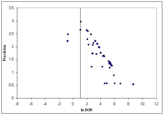
Funnel plot of studies of computer aided detection in mammography, thanks to Leila Eadie

There is an obvious asymmetry and it’s easy to explain. The bottom left corner is missing: small studies that show little or no effect aren’t there. Either researchers don’t bother to write them up, peer reviewers reject them or editors spike them. And you can see why: it’s a small study, and nothing happened.

But there’s a problem. The big studies, the ones that command attention even when the results are disappointing, are hard to fund and hard to complete. The result is that for some hypotheses (say getting children to wave their legs in the air before class makes them clever) we probably only ever see the studies that would be at the bottom right of the ideal plot. How can we judge the true effect?

My conclusion is that there is strong responsibility on those of us who work in fields where there are relatively few large, well-resourced robust studies to be self-critical and to look at how we examine and use evidence to support the claims we make.

Data-mining: it’s all about the data

By rmhipmt, on 4 May 2010

Marooned in NY last week, I made the trek uptown for a meeting at Columbia. It was about data-mining which isn’t really my field, and I might not have gone if the circumstances had been different. It was interesting though, because I think of data-mining as being an applied field of statistics, so assume that the questions are primarily about approaches and involve complex mathematical arguments about the applicability or power of different algorithms or techniques. In this meeting, however, the conversation never got to a mathematical concept more complex than a percentage or a standard test of significance. Instead the discussion was all about the data. What does it mean? How was it gathered? Does it really mean what we think it means?

The project was looking at data about patients who had had an heart attack in hospital. Specifically they were looking at the observations and comments made in the two days before the event to see if there was some signature or pattern that could be used as a warning of the event.

Three interesting observations:

(1) One idea is to look not at the content of observations but at their timing and frequency. In an earlier project the group had assessed the number of comments or observations about a patient. The first pass at that analysis revealed something seemingly odd: a number of patients died without there being anything in the notes to suggest that the patient was ill at all, never mind critically ill. No signs, no symptoms, no tests, nothing. A quick review of the notes for these patient revealed that these were patients who – if not actually dead on arrival – died within minutes. So the absence of information was not a sign of an absence of concern, but that the speed of the crisis altered the requirement for documenting the case.
(2) A previous attempt to identify a predictive signature from the record found that information that was predictive of the outcome wasn’t useful, because it didn’t tell you something you didn’t already know. So, if a doctor orders a test for TB, and this is – to an extent – predictive of TB, well no surprise. The things that were useful – that had been somehow hidden in the data – were only weakly predictive. And how do you use that information clinically? If the test has an AUC that is significantly greater than 0.5 but is only 0.6?
(3) One analysis had involved looking at the comments associated with observations. Unsurprisingly most comments were made about observations that were outside the normal range. Except for oxygen. Most comments about oxygen were made about patients who were in the normal range! So what does that tell us? Well one thing might be that ‘normal’ is a context-dependent term, so that for these patients to be in that range was not normal, or at least was an event that required some documentation.

All in all, it reinforced the impression that health informatics is all about the data. And it doesn’t always mean what it might be thought to mean.

Who decides what we can afford in healthcare technology?

By rmhipmt, on 26 March 2010

Both the major parties acknowledge the need to cut public spending after the election. Neither talks as if cuts are planned to NHS budgets. However, the NHS has always, in its 60 year history, enjoyed real-term increases in spending. A politician promising to protect NHS spending, is rather like someone promising not to halt a rising tide. If the next Chancellor manages to keep the NHS to zero growth, that will seem a huge success. Richard Smith, writing for the BMJ notes that NHS spending has tripled since 1979 and wonders what we have bought for the money: “In 1979 there were about 40 000 doctors and dentists in the whole NHS (it was one NHS in those days) but now there are 122 000 doctors (not dentists) in the English NHS alone. Nurses have increased less dramatically—from 300 000 in the whole NHS in 1979 to 400 000 in the English NHS now. In particular we have many more specialists. Cardiologists were exotic creatures when I was a junior doctor; now they’re a dime a dozen, all busy putting catheters in all day long.”
How did we decide that this level of spending is necessary? It can’t be that we “need” three to five times as many doctors as we did 40 years ago. The answer is that we don’t exactly “decide”. Tony Blair made a conscious decision to increase spending on the NHS, but he was probably responding to public perception of the quality of healthcare here compared to other wealthy European countries, following rather than shaping a public mood. Yet clearly the spending is driven by something, it is a function, somehow, of decisions that are taken by individuals responding to information picked up from contacts and colleagues.
I’ve been talking this week about the move from analogue to digital in breast cancer screening. This hasn’t happened in response to clinical need. Sure, the new machines have advantages over the old, but they don’t offer a step-change in performance. It seems rather that doctors are deciding to buy digital because they are conscious that manufacturers have stopped developing analogue. It doesn’t follow, though, that the process is straightforwardly determined by the manufacturers. The decision to switch to digital can’t have been an easy one for companies with a strong track record in analogue. My guess is that they were trying to provide what they expected customers to want and probably felt that the market was driving the shift. But the astonishing thing is that this cycle – customers making decisions based on what the market offers and the market offering what customers are expected to want – is taking place in a spiral of rapidly increasing costs. Digital mammography is roughly twice as expensive as analogue. Is someone somewhere making the judgement that that’s simply OK? Or maybe lots of people in different places are acting as though that is OK, because it’s hard to see how to act otherwise.